

As part of the Quarterly Report case study, we built a report using the data model, but there were still some instances where we used Excel formulas. In this post, we will be creating a custom field so that there is no need to use SUBTOTAL() formulas for quarterly data!
The Quarterly Report Summary
When we finished the quarterly report, it looked like this:
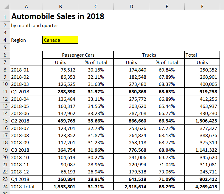
This report shows the listing of units sold of Canadian vehicles by vehicle type and month. The results were taken from a monthly data set of Canadian car sales.
The file at the point where this table has been completed is available for download to get started on adding our new fields in this exercise.
Why do I need custom fields?
In this analysis, we used the SUBTOTAL() function to aggregate our results by quarter. However; this analysis does not fully leverage the power of the data model. In fact, we are doing analysis similar to what was done using SUMIFS().
And what would happen if the report needed to be modified to add only quarterly data, but over a longer span of time, such as 5 years?
To resolve this, we will create a quarterly custom field in the data model to reflect the quarter.
Step 1 – Getting into the data model.
In order to create the custom field for quarters, first you will need to get into the data model. This is located under Power Pivot, manage Data Model.

This option will get you right into the data model, where all the data resides!

Step 2 – Name a Custom Field
At the end of the columns, there is a blank column for creating new columns.

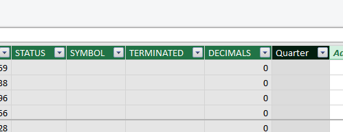
When we double click on the option to add a new column, it allows a new column to be created. In this case, the new column will be named “Quarter”.
Once the new column is created, it is identified as being a custom field by the fact that it is in black, whereas all the other columns are in green.
Step 3 – Create the Custom Field Formula
Returning to our original data, the quarters appeared as “quarter-number year”. This is not a number, so we will need to parse this together from our REFDATE field, which does show the date.

There are 3 formulas that are required in order to parse this date; ROUNDUP(), MONTH() and YEAR().
Note – all 3 of these functions can be used in Excel, and are not specific to the Data Model.
Required Functions for Quarter Parsing
MONTH(Date)
This formula takes a date, and provides the month.
=MONTH("March 1, 2018")
3
YEAR(Date)
This formula takes a date, and provides the month.
=MONTH("March 1, 2018")
2018
ROUNDUP(Number, Number of Digits)
This formula takes a number and rounds it up to a specific number of digits, as determined in the formula. In order to round to the nearest whole number, select 1 digit.
=ROUNDUP(10/3,1)
4
How do I use the formulas to pick the quarter?
Start with a “Q”
First, all quarters start with the letter “Q”. After that, add a & symbol to concatenate the quarter number.
="Q"&Add the Quarter Number
The quarter number is calculated based on the REF_DATE field.
First, calculate the month that the date belongs to, and divide the date by 3.
An example when the REF_DATE is February 1, 2018:
=MONTH(CarSales[REF_DATE])/3
0.666666
Next, round that number up to the nearest whole number.
=ROUNDUP(MONTH(CarSales[REF_DATE])/3,1)
1
At this point, our formula should look as follows. After adding the quarter number, it is required to add a blank space before adding the year.
="Q"&ROUNDUP(MONTH(CarSales[REF_DATE])/3,1)&" "&Finish with the year
Finally, add the year to the formula.
="Q"&ROUNDUP(MONTH(CarSales[REF_DATE])/3,1)&" "&YEAR(CarSales[REF_DATE])When all of this is complete, your custom field should show the quarter the same way that it appears in the report!

Step 4 – Add the Quarter custom field to the report
If you return to the CUBEVALUE() formula, you will now notice that the Quarter field is now available for selection.

Instead of retyping the entire formula, copy one of the monthly formulas to cell B11. Then, change the [CarSales].[REF_DATE] reference to [CarSales].[Quarter]. Your formula should now look like this:
=CUBEVALUE("ThisWorkbookDataModel","[Measures].[CarSalesTotalValues]","[CarSales].[UOM].[Units]","[CarSales].[Origin of manufacture].[Total, country of manufacture]","[CarSales].[GEO].["&$B$4&"]","[CarSales].[Quarter].["&$A11&"]","[CarSales].[Vehicle type].["&B$6&"]")After adjusting the formula for Q1 2018, copy the new quarterly formula to all of the other quarters on the page.
Step 5 – Removing SUM() and modifying other totals
Now that you are comfortable fixing a filter to add a custom field, there are some other cells that can be modified by removing filters entirely.
Column Totals
A column total removes the filter for the dates completely. In the case of cell B24 (the total for passenger cars), it is as follows:
=CUBEVALUE("ThisWorkbookDataModel","[Measures].[CarSalesTotalValues]","[CarSales].[UOM].[Units]","[CarSales].[Origin of manufacture].[Total, country of manufacture]","[CarSales].[GEO].["&$B$4&"]","[CarSales].[Vehicle type].["&D$6&"]")Row Totals
A row total removes the vehicle type filter, but keeps the filter for the date. In the case of F11 (total for Q1 2018).
This should work as follows:

Notice – in this case, it does not work as expected. This is because in our underlying data, there is a “Total, new motor vehicles” option. While there are ways to filter this out, we will explore this more later.

Next Steps
There are 2 next steps that will dig a bit deeper into the data model.
- The percentage of total field – this will require some more advanced calculations than just a SUM(); this will be a new calculated measure!
- Getting rid of totals – there are a few ways to fix the totals that we don’t need for this analysis that will be explored!