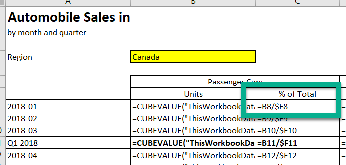
In the last post, we started using the CALCULATE() function to filter out some of the values that we didn’t want on our totals. This was done in order to get a pivot table that didn’t need to use the SUM() function to add up the values on the sheet.
The only values that are left on the sheet that are still being calculated by Excel are the percentages of the total row.
We will be using the Canadian Car Sales model that uses data available from Statistics Canada and is available on this site.
What we have done so far…
In prior exercises, a table for calculating car unit sales by month, quarter, region and vehicle type was created.

This table used:
- A custom measure in the data model to get the sum of all cars.
- The CUBEVALUE() function to take the values out of the data model.
- A custom field to determine the quarter that the cars are sold in.
Looking at the functions for all the values, the only cases where the CUBEVALUE() function is not used is on the percentage of total cars for the row.

In this exercise, we’ll introduce the ALL() function and create a new custom measure to easily perform this calculation!
This post assumes that you have already created the data model in the prior exercises. The version of this file needed to start this exercise is available at:
Example of CALCULATE()
Why can’t we just divide 2 CUBEVALUE() functions?
There is nothing really stopping you from using the existing CUBEVALUE() function, then dividing that by the CUBEVALUE() function in the total cell.
The code for that function is below.
=CUBEVALUE("ThisWorkbookDataModel","[Measures].[CarSalesTotalValues]","[CarSales].[GEO].["&$B$4&"]","[CarSales].[REF_DATE].["&$A8&"]","[CarSales].[Vehicle type].["&B$6&"]")/CUBEVALUE("ThisWorkbookDataModel","[Measures].[CarSalesTotalValues]","[CarSales].[GEO].["&$B$4&"]","[CarSales].[REF_DATE].["&$A8&"]","[CarSales].[Vehicle type].[Total, new motor vehicles]")However; this code is very inefficient. Instead of using the CUBEVALUE() formula, we can perform this calculation directly in the data model.
Adding the new CALCULATE() measure.
New measures are located under the measures menu under the Power Pivot menu.

In this example, we will be creating a new measure in order to calculate the percentage of a row.
This will bring up the screen to add a new measure. This new measure will be to calculate the percentage of all car sales, based on the vehicle type.

Introducing the DIVIDE function
While very unlikely in this case, there are some cases where there could be no results for a month. This would cause the denominator to be zero, and would bring up errors in our calculations! A method to get around this issue is using the DIVIDE function.
The DIVIDE function:
Performs division and returns alternate result or BLANK() on division by 0.
https://docs.microsoft.com/en-us/dax/divide-function-dax
This ensures that there is no possibility of having an error in our results. The DIVIDE function is created as follows:
=DIVIDE(numerator, denominator, alternate value on zero divide)In our quarterly report:
Numerator – the number of cars sold for a vehicle type.
Denominator – the number of cars sold for all vehicle types.
Alternate Result – will be zero.

Adding the existing Car Sales measure.
When we build the new function to divide the individual monthly data points by the total, we don’t have to reinvent the wheel! In this case, we can start with the CarSalesTotalValues measure as the numerator.

We can continue using the CarSalesTotalValues measure for our denominator as well, but we need to provide an additional CALCULATE function to get this working properly!
This is where the ALL function will be required.
Introducing the ALL function
The ALL function allows us to override a filter that may already be in place; in this case, the filter on vehicle type. Or, as it is officially explained, it:
Returns all the rows in a table, or all the values in a column, ignoring any filters that might have been applied. This function is useful for clearing filters and creating calculations on all the rows in a table.
https://docs.microsoft.com/en-us/dax/all-function-dax
In order to calculate the percentage of sales by vehicle type, we need to be able to calculate the whole row as the denominator.
If used within a CALCULATE function, the ALL function acts as a kind of negative filter; instead of filtering for results, it removes existing filters.
CALCULATE(Measure, ALL(column to include all values))In this report, we will use the CarSalesTotalValues measure, removing the Vehicle type using the ALL function to create our denominator.

Finally, we will add in the zero alternate result and close off the DIVIDE formula.

To ensure that there are no issues with the formula, we can make a final check by clicking on Check formula. After verifying that there are no errors, click OK to create the new measure.

Adding the new measure to the CUBEVALUE formula.
Since the new measure uses the same fields as the existing measure, we can use the same CUBEVALUE formula; the only thing we need to change is the measure!
Copying the values from cell B8 into cell C8 will provide the same value in cell C8; the only difference is that it shows as a percentage!

However when we click on the measures in the CUBEVALUE formula, we can now add the new PercentageofCarSales measure into the CUBEVALUE formula.

After modifying the measure in the CUBEVALUE formula, the correct percentage of total displays in the cell!

Voila! After copying this new formula to the rest of the cells where the division was being done in the cells, every formula is now being calculated using CUBEVALUE.
Next Steps
Since there are no longer any formulas that are reliant on Excel cells, the next step could be to create the table in Power BI.
Alternatively, the sheet could be improved in order to make sure that users can’t modify the sheet to break all the formulas!

