Cube formulas have been around in Excel for a long time. Not like VLOOKUP (which has been around since the beginning)… but they have existed since 2007. These formulas were initially designed to extract values from SSAS cubes.
However; with the introduction of Power Pivot in 2010, these formulas have become much more valuable. Now, you have a full data model within your spreadsheet!
An example of using the CUBEVALUE() formula is available in the Quarterly Report case study; however, this posting will go into greater detail as to why you might want to use a cube formula, as well as some additional tools to help build cube formulas.
Why do I want to use cube formulas?
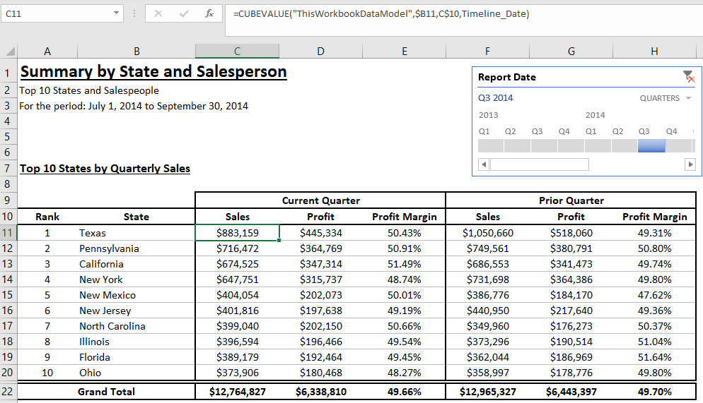
In the example below, we have a spreadsheet where a PowerPivot has been created to summarize the top 10 sales results in a quarter by state.
This sheet is available on this site:
The model requires the Wide World Importers database available from Microsoft.

While this may provide the required information:
- The amount of formatting that can be applied is limited. Pivot tables only allow for a limited amount of customization to formatting.
- Sorting must be done by a known field or measure. In some cases, sorting needs to be in an arbitrary manner (e.g. on a balance sheet – assets are ordered by liquidity).
- A full pivot table may be required to extract a single value, such as the date between the selected slicer.
- Measures (such as the rank, which uses the RANKX() DAX function) cannot be placed before columns. This can force some inefficient calculated columns if they need to appear in the first column!
Since a PivotTable is sometimes not the best solution, how can these issues be resolved while still having a data model? The answer is cube formulas.
How can I get started with cube formulas?
If you have created a Power Pivot from a data model, there is a tool under PivotTable Analyze > OLAP Tools. This will convert the Power Pivot into formulas – every cell can be moved on the spreadsheet!

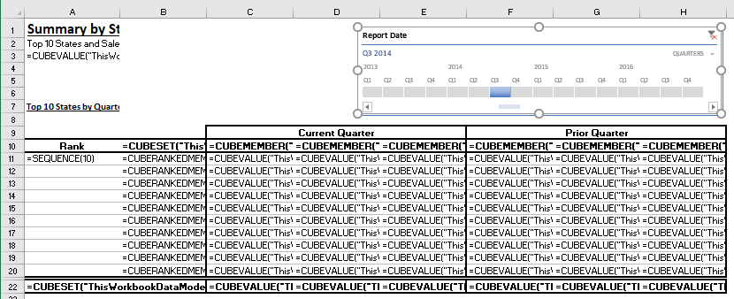
After converting the pivot table to formulas, the new report should look identical to the pivot table that existed before the conversion to formulas!

However; if you were to view formulas on the spreadsheet – you will see that the pivot table is actually all cube formulas!

But what do all these formulas mean?
The 4 Cube Formulas in the Example
There are 4 cube formulas that are used in the example above:
- CUBEMEMBER() – This formula extracts a member from a cube; either a measure name (such as Sum of State Sales) or an element from a column in a table (such as Texas, from the geography table, in the State column).
- CUBEVALUE() – This formula will calculate a value directly from the data cube based on parameters that passed into the formula, including cube members or slicer values.
- CUBESET() – This formula extracts all unique values from a set expression, and can apply a sort based on . Normally this will be a single table column when working with the Excel data model.
- CUBERANKEDMEMBER() – This formula extracts the member that is at a specified position within a set defined by a cubeset formula.

CUBEVALUE() – Using as a Header
In order to add a header with the dates from a slicer, first a simple DAX measure is created:
Selected Dates := "For the period: "&FORMAT(min('Dimension Date'[Date])
,"mmmm d, yyyy") & " to " & FORMAT(max('Dimension Date'[Date]),"mmmm d, yyyy")
If you want to add the date from a selected slicer to a spreadsheet using a pivot table, an additional row will be added above the measure. There is no way to remove this blue row.
If a pivot table is used, the best solution is to hide this row, or incorporate the title into your design.

However; you want to be able to add just the date values! In this case, we will add the CUBEVALUE() formula.
CUBEVALUE() Syntax
=CUBEVALUE("ThisWorkbookDataModel","[Measures].[Selected Dates]",Timeline_Date)The CUBEVALUE() formula consists of 3 elements:
- The connection – In an Excel data model, this will always be ThisWorkbookDataModel.
- A measure – This is what the cube value is aggregating.
- Additional cube members or slicers – These will act as filters on the measure.
In our first example, we are only filtering based on a timeline, though other examples will filter based on cube values.
To use the Excel data model, the connection will always be the “ThisWorkbookDataModel” connection. When typing the connection string, Intellisense will auto-fill this connection after entering a double quote. This will only be different if the connection is to an SSAS model.

After adding the connection string, all measures can be located by selecting Measures. Intellisense will locate the required measure after Measures are selected.

Finally, a slicer can be added into the CUBEVALUE() formula. Unlike adding a measure or table field, slicers do not use a double quote to add the slicer. However; Intellisense will locate all the slicers so they can be properly added to the formula.

This formula will show the period that has been selected by the slicer without the need for a pivot table!

CUBEMEMBER() – Adding a Field or Measure
When a Power Pivot is converted to formulas, the measures and table fields are converted into CUBEMEMBER() formulas.

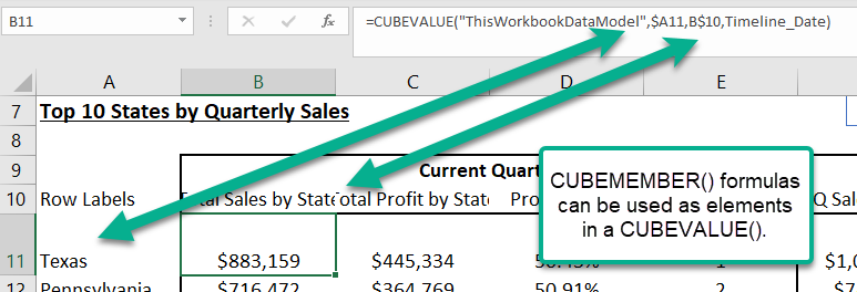
These formulas can be used in cell references when building up CUBEVALUE() formulas. As a result, using CUBEMEMBER() can make CUBEVALUE() formulas much more readable!

CUBEMEMBER() Syntax
=CUBEMEMBER("ThisWorkbookDataModel","[Measures].[Total Sales by State]","Sales")The CUBEMEMBER() formula consists of 2 required elements and 1 optional element:
- The connection – In an Excel data model, this will always be ThisWorkbookDataModel.
- A measure or table field.
- An alias (Optional) – If the name of the measure or table field is not in a user readable format, this can be overridden to a more useful name.
An example of the Alias field is when a measure name is in a format that doesn’t make sense for the report that is being built. Or, if the measure name is not designed to be seen.
The measure “Total Sales by State” has a redundant name, and could make the summary hard to read.

The alias “Sales” makes the field much easier to work with!

CUBESET() – Adding and Sorting Table Values
The CUBEMEMBER() formula is great for adding members that do not change frequently, or measures that do not change at all.
However; in most real world scenarios, data is added to columns. Or, columns need to be sorted alphabetically or numerically.
This eliminates the need to add all potential values as CUBEMEMBER() formulas; they can be taken from a pre-defined set of values in the spreadsheet!

This formula does involve a more complex syntax, so it may not be the answer all the time!
CUBESET() Syntax
=CUBESET("ThisWorkbookDataModel","[Dimension City].[State Province].children",
"State",2,"{([Measures].[Total Sales by State],
[Dimension Date].[Calendar Quarter].[CY2014Q3])}")
The CUBESET() formula consists of 2 required elements and 3 optional elements:
- The connection – In an Excel data model, this will always be ThisWorkbookDataModel.
- A set of items – in MDX format. I’ll explain this below.
- An alias (Optional) – If an alias is not used in this formula, the cell will show as blank. The cell will still show #N/A if there is an error.
- A sort order (Optional) – If this is used, data can be sorted alphabetically or numerically.
- Sort by (Optional) – If the field needs to be sorted by another value (i.e. States need to be ordered based on sales), this can be used to determine the field for sorting.
What is a valid set of items?
There are normally 2 types of items that you can add as a set in Excel. While more complex MDX expressions can be used, these are not required.
- A slicer – In the example below, the CUBESET() takes all selected values of the slicer. The slicer name, Slicer_State_Province is used to define the active slicer.

2. A field in the data model – Normally, when using a CUBESET() formula you will use a field in the data model.
The major difference is that in order to create a proper MDX expression, you need to add .children at the end of the item set. This will not be shown automatically (with Intellisense) when you enter the formula.
This will return an error:
"[Dimension City].[State Province]"But this will return a list of all unique states in the [Dimension City] table:
"[Dimension City].[State Province].children"
How can I sort my set?
Data will appear in the order that it appears in the data set by default. However; one of the great powers of the CUBESET() formula is that it can sort values automatically.
There are several different options for sorting using a number for the Sort Order parameter. Normally, you should use Natural Order for numerical data – otherwise, it will sort numbers as letters!
The sort by parameter requires more explanation.
| Parameter | Option | Example |
|---|---|---|
| 0 | No Sort | 7,1,23,12,21 |
| 1 | Ascending (based on Sort By) | *** |
| 2 | Descending (based on Sort By) | *** |
| 3 | Alphabetical (Ascending) | 1,12,21,23,7 |
| 4 | Alphabetical (Descending) | 7,23,21,12,1 |
| 5 | Natural Order (Ascending) | 1,7,12,21,23 |
| 6 | Natural Order (Descending) | 23,21,12,7,1 |
How does the Sort By work?
By selecting sort order 1 (ascending) or 2 (descending), an additional criteria can be chosen for sorting.
Sort by allows the set by another column or measure, such as sorting states based on sales.
=CUBESET("ThisWorkbookDataModel","[Dimension City].[State Province].children",
"State",2,"[Measures].[Total Sales by State]")
To sort values by a single measure, the measure can be provided in quotes.

However; this measure will apply against the entire data set! If there are any slicers in place, they will not be used in the CUBESET() formula!

How can a slicer be applied to a CUBESET() formula?
In order to use a slicer, a second value needs to be added to the added to the sorting criteria. This will filter the table based on the secondary criteria.
=CUBESET("ThisWorkbookDataModel","[Dimension City].[State Province].children","State", 2,
"{([Measures].[Total Sales by State], [Dimension Date].[Calendar Quarter].[CY2014Q2])}")
Some important things to know about adding a second criteria:
- All criteria needs to be enclosed in curved and normal brackets {[ ]}.
- A slicer cannot be directly added to a sort.

Since you cannot directly add a slicer to the CUBESET() formula, a simple DAX measure needs to be created to extract the active quarter.
Selected Quarter := MIN('Dimension Date'[Calendar Quarter])Then, the value from this measure can be extracted directly from the spreadsheet (assuming that the new measure is in cell A4).
=CUBESET("ThisWorkbookDataModel","[Dimension City].[State Province].children","State", 2,
"{([Measures].[Total Sales by State], [Dimension Date].[Calendar Quarter].["& A4 &"])}")
This provide the values we want, in the order we expect!

CUBERANKEDMEMBER() – Extracting Values from a Set
The CUBERANKEDMEMBER() formula is used when there is a cube set already defined on the spreadsheet. This allows the values to be extracted from the cube set into individual cells.

CUBERANKEDMEMBER() Syntax
=CUBERANKEDMEMBER("ThisWorkbookDataModel",$B$10,A12)The CUBERANKEDMEMBER() formula consists of 3 required elements and 1 optional element:
- The connection – In an Excel data model, this will always be ThisWorkbookDataModel.
- A valid cube set – This will be the cell containing the CUBESET() formula.
- The rank within the set to extract – This can be a cell reference or a hard coded value.
- Alias (Optional) – This should be used if you want to override the default value that is returned from the cube set (e.g. you want “Top Performer” as the #1 value).
The CUBESET() formula does most of the work when it comes to filtering and sorting values in the cube!
CUBEVALUE() – Using with CUBEMEMBER() and CUBERANKEDMEMBER()
If cells contain CUBEMEMBER() formulas and CUBERANKEDMEMBER() formulas, these can be used as elements in a CUBEVALUE() formula.

=CUBEVALUE("ThisWorkbookDataModel",$B11,C$10,Timeline_Date)In this example, cell B11 does not contain the value “Texas”. It contains a CUBERANKEDMEMBER() formula that returns the value Texas. As a result, the CUBEVALUE() can use this cell as a filter in the formula.
Likewise, cell B10 does not contain the value “Sales”. It contains a CUBEMEMBER() formula with the Total Sales by State measure which has the alias Sales.
Finally, the CUBEVALUE() is filtered by active values in the Timeline_Date slicer.
This returns the sum of sales for the top ranked state in Q2 2014!
Conclusion – Is there a reason to NOT use cube formulas?
Cube formulas can be a powerful way to ensure that data is extracted from a cube into a spreadsheet in a precise, presentable format.
However; if a pivot table can be used, a pivot table should be used.
Cube formulas are less efficient (they require greater calculation time), and use more complex syntax than pivot tables.

