When receiving a list of data, it can be desirable to find unique values. This can be accomplished in Excel using the UNIQUE() function, or by using other methods for getting unique values. But, what happens if you’d like a list of only values where there are duplicates?
There is no function in Excel to automatically create a list of non-unique values. However, with a combination of some existing functions, we can create a way to get a list of all duplicates in a an existing list.

The Example File
The example file that we will be using is a list of 100 random generated names. While all the names in the file are unique, some of the first names are duplicated.
The Formulas To Use
There are 3 formulas that need to be used in order to build this list. In order to use these formulas, you will require one of:
- Excel 365
- Excel 2021
COUNTIF() – This function will be required in order to determine if a name is unique or not.
FILTER() – This function will be used to remove unique values.
UNIQUE() – Once we have a list of duplicates, remove the duplicates from the duplicate list.
Find the Duplicates – The COUNTIF() Function
The first function that is required in this example is the COUNTIF() function. The COUNTIFS() function can also be used, but is not required in this example.
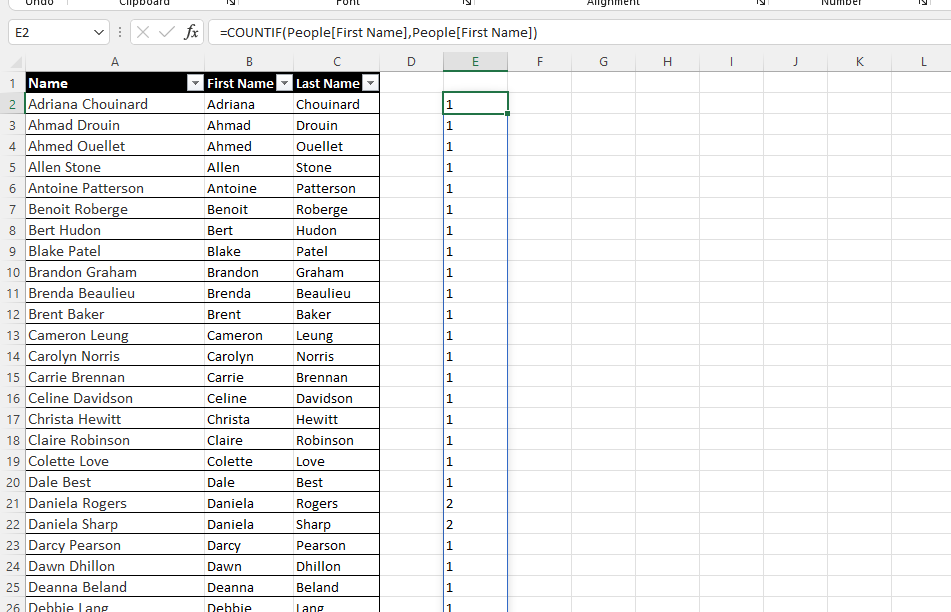
For this COUNTIF(), we are looking to determine how many times a first name appears, for each first name that is available.
So, we actually need to use the same argument twice. The first will determine the list of names, and the second will give a list of names to compare against.
=COUNTIF(People[First Name], People[First Name])This will build an array for every first name in the list showing how many times the name appears in the list, like the image below. Note that while most appear 1 time, Daniela appears twice.

Filtering Out the Unique Values – The FILTER() function
Once we can determine which of the names are duplicates, the next step is to use the FILTER() function to return a list of names which are duplciates.
The FILTER() function requires 2 lists – the first is the list to be filtered, and the second list is an equal length list which is either true or false.
Let’s take a look at how this works.
=FILTER(People[First Name], COUNTIF(People[First Name],People[First Name])>1)For each person’s first name, the COUNTIF() function provides a number. If that number is 1, the name is unique. If it is over 1, it is not unique.
By checking if the value is over 1, unique values will show as FALSE, whereas non-unique values will show as TRUE.

The FILTER() function will remove any values which are FALSE, returning a list of only the names which are non-unique. However; there is one more step to remove the duplicates from the list!

Use UNIQUE() to Remove Duplicates Within the Duplicate List
While the list of values contains only values where there is duplication, the names appear more than once – the filter returned every case where a duplicate exists!
To show only 1 case of each duplicate value, you can wrap the entire formula in a UNIQUE() formula.
=UNIQUE(FILTER(People[First Name],COUNTIF(People[First Name],People[First Name])>1))This will show a list of every value where there is a duplicate – but only once!

Conclusion – Limitations and Adding Reusability with LAMBDA()
In the example provided, the formula is only looking for duplicates within a single column. Looking within multiple columns is more challenging. It can’t be solved simply by using the COUNTIFS() function!
If the formula needs to be used for multiple columns or ranges, it can be worthwhile to consider using a LAMBDA() function. The code for creating your own duplicates LAMBDA() function is below!

LAMBDA(list,
    unique(
        filter(
            list,
            countifs(
                list,
                list
            ) > 1
        )
    )
) 
