
There are many times where you will need to acquire a unique value from not just one list of values, but from two separate lists.
Getting a unique value from a single list is straightforward, and can be accomplished in Excel using the UNIQUE() function in Excel.
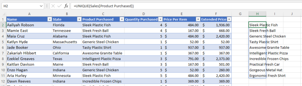
The UNIQUE() function can take a single column, and extract unique values from the column.
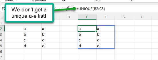
However; when there are multiple columns, the UNIQUE() function will look at the entire set of data, and will look row-by-row. This will not provide a usable unique list!
We will be looking at 3 methods to get unique values from two separate columns using the following methods:
- Using the Remove Duplicates option to get unique values.
- Creating a new table in Power Query with unique values.
- Combining VSTACK() and UNIQUE() to provide a unique list.
The Data – The Problem!
In the case that we’ll be looking at, there are 2 tabs on the spreadsheet, which in a real world scenario might represent data which comes from 2 different systems and requires reconciliation.
This data is available in the download below:
The first is Total State Sales, which would represent a system that looks at sales in aggregate – such as a general ledger system.

The second is Sales, which provides a transaction by transaction view of sales over the period of time.

An analyst may be assigned to reconcile the 2 systems, to ensure that all sales that are in the transactional system are represented in the system which aggregates by state.
So, the analyst proceeds with using a SUMIFS() formula to sum the extended price by state. This will be compared against the total value on a state by state level. The variance column shows no variance, so the job is done! Right?

Not so fast! When looking at the sum of the Sales table, there are $1,026 in transactions which are not included in the state by state calculations!

Further investigation shows 3 transactions which did not show up on the state table:
- 1 transaction from Washington D.C. which did not show up because of inconsistent formatting.
- 2 out of country transactions from Canada and Mexico which would not show up on the state table.

So, how can we solve this problem? By using a process that gets unique values from both tables.
Getting Unique Values using Remove Duplicates
A simple way to get unique values from a list where the values will not change is to use the Remove Duplicates functionality, which can be found under the Data menu.

First, copy the State column from one of the two data sets. I’ll use the Sales tab in my example.

Then, copy the data from the other data set underneath the data from the first data set. Make sure not to include the State header, because it would be included in your data!

Once all the states have been added. select the top of the new State column and click Remove Duplicates. The “My data has headers” option should remain checked. Then, click OK.

This will provide you with a unique list of states from the combination of both lists. This list will be unsorted, and the formatting will remain from before duplicates were removed.

Getting Unique Data using XLOOKUP
Since each value on the Total State Sales table is unique, you can use an XLOOKUP (or VLOOKUP) function to get values from the Total State Sales table.
=XLOOKUP(A2,StateSales[State / Region],StateSales[Total Sales],0)If using the XLOOKUP function, make sure to add the 0 as an optional argument after selecting Total Sales as the default. There will be some values that are not on the state table that we wouldn’t want to show up as N/A!

Getting Non-Unique Data using SUMIFS
Since there are multiple references to the same state on the Sales table, the XLOOKUP formula cannot be used.

Instead, we’ll use the SUMIFS function to get the extended price from the Sales table.
=SUMIFS(Sales[Extended Price],Sales[State],A2)
Once the data from the sales table has been added, add a variance column by subtracting one column from the other.
Formulas can be filled down by selecting the 3 columns and double-clicking the bottom right corner of the range.

Once this is done, the cases where the state is not on the state table are clearly visible!

Getting Unique Values using Power Query
If the data that you are working with comes from an external file, or changes more frequently, a more efficient approach to getting unique values is available using Power Query.
Before getting started, your data needs to either be:
- In a table in your Excel file
- In an external file / database.
For this example, we’ll be using two tables which are in the demo Excel file. Each table will be loaded into Power Query using the From Table/Range option.

There should be 2 tables in Power Query before getting started – Sales and StateSales.

Getting only Unique Values from Power Query
In order to just get unique values, we will follow a similar process that we followed with Remove Duplicates. That is, we will stack the states on top of each other, and then get distinct values.
However; before getting unique values from Power Query, the state columns need to be the same name.
Renaming the State Column

In the State Sales table. the State column is named State / Region.

To rename the column, right click on the column, then select Rename and enter State as the new name for the column.

Once the columns have the same name, the tables can be stacked on top of each other in order to get unique values.
Stacking Tables to Get Unique Values
To create a new query, select the option to “Append Queries as New”

Each of the 2 tables needs to be selected for the Append query. It doesn’t matter which table is selected as the first query and which is selected as the second query.

This will create a new view, Append1 which has every unique field from each table – but since the State field is unique, it will stack the fields on top of each other.

Once this is accomplished, remove all the other columns other than the State column. This can be done by selecting the State column and picking Remove Other Columns.

To make sure that only a unique list of states is left, click on Remove Duplicates under the Remove Rows option.

Finally, rename the query and load to the spreadsheet.

Create Totals on Spreadsheet from Unique Values
Once the table is loaded to the spreadsheet, the totals by state and by transaction can be added based on the unique values.
The only difference versus the earlier method where stacking was used is that the formulas refer to a row ([@State]) as opposed to a cell (A2).
Getting Values from the Total By State Table
=XLOOKUP([@State],StateSales[State / Region],StateSales[Total Sales],0)
Getting Values from the Sales by State Table
When working with the Sales table, like earlier, you need to use a SUMIFS formula as there are multiple instances of the same state when working with states.
=SUMIFS(Sales[Extended Price],Sales[State],[@State])
Finally, once you have values from both tables, you can subtract one column from the other.

Finding Unique Values using VSTACK()
If you have access to the most recent version of Office 365, you can use the VSTACK() function to append one table to the bottom of another.
In this case, we will be using the VSTACK() function on the State column to capture a list of all states in both tables; like we did with the Remove Duplicates functionality – only this time, we’ll do it only using formulas!
Using VSTACK() to Append One Column on Another
Using the VSTACK() function, select the State column from both of the tables. The two tables can be in any order; we will be dealing with sorting later.
=VSTACK(Sales[State],StateSales[State / Region])
This will create a single column containing the state on every row in both the sales and the sales by state tables.
However; at this point, while the state columns are stacked on top of each other, there are duplicate values.

Remove Duplicates Using the UNIQUE() Function
In order to remove duplicates from the stacked column, the function needs to be wrapped in a UNIQUE() function. This formula will ensure that every value from the stacked tables is unique. There is no need for any optional parameters on this formula.
=UNIQUE(VSTACK(Sales[State],StateSales[State / Region]))
Sort Values Using the SORT() Function
Although there are only unique values in the list, they are in the order that they appear in the initial data source (which may just be the order in which the sales occur!). To provide a more relevant set of results, the values will be sorted alphabetically by wrapping the values in the SORT() function.
=SORT(UNIQUE(VSTACK(Sales[State],StateSales[State / Region])))
Create Totals from Dynamic Unique Values
Once the list of unique states has been created, the XLOOKUP() and SUMIFS() formulas will need to be used to create the values by state.
However; since the list of states has been created dynamically, you can use a # (hashtag) to create a calculation for each different value in the column!

Getting Values from the Total By State Table Using the Hashtag
The XLOOKUP formula will be the same as the ones earlier; the only difference is that instead of referring to just cell A2, we will refer to the entire state range using A2#.
By using the hashtag, we can get all values by state looked up on a row by row basis.
=XLOOKUP(A2#,StateSales[State / Region],StateSales[Total Sales],0)
Getting Values from the Sales Table Using the Hashtag
For the SUMIFS() formula, the same pattern can be followed. The A2 cell reference can be replaced by an A2# reference to refer to the entire cell range.
=SUMIFS(Sales[Extended Price],Sales[State],A2#)
Once values from the total table and the transaction table have been added, you can subtract one column from the other on a row by row basis using the hashtag.
=B2#-C2#
Conclusion
With the addition of Power Query and the VSTACK() function, there are more and more ways to be able to get unique values from two different sets of lists.
But when should we use each method? While there are some firm rules around not being able to use some functionality if was not available in the version of Excel, there are some suggestions around when to use each method.
Remove Duplicates
- The analysis is being done in Excel 2013 or earlier.
- It is unlikely that the data will need to be refreshed; there is little chance for new unique values to be required.
Power Query
- The analysis is being done in Excel 2016 or later, but not the latest version of Office 365 (the VSTACK() function is still beta as of May 2022)
- The values are being acquired from an external source, and may change frequently.
VSTACK()
- The analysis is being done in the latest version of Office 365.
- The data in question is not in a table format usable for Power Query.
- Data is stored in the sheet (or needs to be shown outside of the data model).